• Background
• How molecular dynamics works
• The experiments: Atomic force microscopy
• What we actually did: Observing the binding modes
• Measuring bend angles
• Sequence specificity
• Investigating the asymmetry using free-energy calculations
• DNA bridging by IHF
• A complete model of IHF binding, bending, & bridging

The first paper from my PhD has finally been published! Using an exciting combination of advanced simulations and microscopy, the paper reveals the multiple ways in which a protein found in most bacteria bends DNA and demonstrates that the protein can hold together two separate DNA helices. This has some important consequences for our understanding of DNA organisation in bacteria and the stability of infectious bacterial colonies, and the tightly coupled combination of experiment and simulation presents a promising foundation for future studies into other important biological systems. Unfortunately, a scientific paper is by its very nature a relatively dry, technical document, but the fruits of science belong to us all and I think it’s important that we share our research outside the academic bubble. With that in mind, please do sit tight while I walk you through our work in terms I hope a scientifically curious layperson can understand.

---

For those who want to skip straight to the paper, it’s published (open-access) in Nucleic Acids Research—the full citation is

Yoshua S B, Watson G D, Howard J A L, Velasco-Berrelleza V, Leake M C, Noy A 2021 “Integration host factor bends and bridges DNA in a multiplicity of binding modes with varying specificity” Nucleic Acids Research gkab641 doi:10.1093/nar/gkab641

My role in the project revolved around the simulations—I set them up, ran them, fixed them when they went wrong, and analysed the results. Dr Sam Yoshua did the same for the experimental portion of the project, and we’re considered joint first authors, however little sense that phrase may make. My portion of the work is discussed in more detail, with more in-depth explanation of the methods, in my PhD thesis, and Sam’s in part of his. Meanwhile, Dr Agnes Noy and Prof. Mark Leake designed much of the project, secured funding, and provided invaluable support and expertise throughout.

A final note before we begin: While Sam and I created the vast majority of the images in the paper, the copyright is now held by Oxford University Press, publishers of Nucleic Acids Research, who have very kindly granted permission to use them under a Creative Commons Attribution (CC-BY) licence. It is under those terms that I share my own work here.¹

If you feel like you already have a good understanding of DNA, proteins, molecular dynamics, and atomic force microscopy, feel free to skip right to the results. Otherwise, I’ll do my best to give you the background knowledge you need.

Right, onto the good stuff!

Background

I’m sure you already have at least a vague grasp of what DNA is. It is perhaps the single most important and interesting molecule in the universe, for it contains all of the information that makes (most known) living things what they are. Composed of two very long strands held together by paired “bases” containing the genetic code, and neatly packaged into the iconic double helix, the storage and maintenance of DNA is a perpetual problem for all life.

The problem is, one must store a lot of information to make a functioning organism—the human genome consists of around 6.4 billion base pairs with a total length of around two metres. And there is a separate copy of that genome in every one of your cells,² each of which has a diameter of less than 100 micrometres. These numbers are not easy to comprehend, but the point is that genome packaging is a very important and difficult problem. How do you fit that much DNA into a cell while still ensuring you can access the bits you need when you need them?

Eukaryotes—complex organisms like plants and animals—have converged on a complicated solution to this problem, involving the wrapping of DNA around special proteins called histones. Bacteria have their own solution, involving a range of “histone-like” proteins collectively called “nucleoid-associated proteins” (NAPs), which bind to DNA and wrap it around themselves.

Of course, bending DNA like this affects how it behaves. Some DNA is easy to access, allowing it to be read, processed, and used to make proteins, while other DNA is inaccessible to the cellular machinery. Understanding how DNA is packaged, and the factors affecting this, means being able to predict and control which genes will be expressed and when. To understand this better, we studied one of these proteins, called integration host factor (IHF), which is common across a wide range of bacteria and has a lot of features that make it a good example of a general NAP. IHF creates sharp U-turns in DNA, bending it back on itself by about 160°, but (spoiler alert) I’ll soon reveal that there’s more to the story than that.

Another interesting thing about IHF is its presence in some bacterial biofilms—sticky colonies of bacteria surrounded by a protective matrix that makes them particularly pernicious pathogens, causes a lot of problems when they get into your body, and enhances their resistance to antibiotics. In some of these biofilms, large amounts of DNA and proteins are pumped out of the cells, forming a three-dimensional scaffold of DNA strands that supports the structure. IHF is often found at the points where these strands cross, and removing IHF causes the biofilms to collapse. How does IHF perform this important role in stabilising biofilms?

To answer these questions, I worked closely with Sam to develop a set of simulations and experiments that work in parallel to complement one another. My part of this was a simulation technique called molecular dynamics, which uses supercomputers to simulate the movements of each individual atom making up a biological system, while Sam used a technique called atomic force microscopy (AFM), which uses a tiny needle to trace the surface of an object and construct a detailed heightmap. If you just want the biology, feel free to skip the next couple of sections, but I think it’s valuable to understand the way in which these results came about, so I’ll try to give you a brief overview of (my understanding of) these techniques next.

How molecular dynamics works

Molecular dynamics (MD) simulations are a favourite technique of mine. I provide a detailed technical overview in chapter 2 of my thesis, but I’ll give a briefer overview in terms normal humans can understand here.

MD is a way of modelling the movements of atoms and molecules by simulating their movement over a series of very short time steps. After providing an initial structure, the basic steps are:

1. Calculate the force between every pair of atoms, and how much they should be accelerating.
2. Move the atoms by the amount they should move in our small time step.
3. Make sure everything stays in the box.
4. Repeat lots and lots³ of times.

That makes it sound easy, but each of these steps hides a lot of complexity. Lots of things can affect the force between two atoms, but the most important are:

• The distance between them—too close and they’ll repel each other strongly; too far apart and they’ll be gently attracted to each other
• Their charge—like charges repel each other, while opposites attract
• Covalent bonds—these are what hold molecules together, and come with complicated restrictions on lengths and angles

There are a huge range of force fields that model these interactions,⁴ and people keep tweaking them to make the results even more accurate. There are a lot of other forces that you might be surprised to see excluded, like gravity; in reality, these are simply far too weak at these scales to make any difference to the system, and it would be a waste of precious computation time to calculate them.

The other big problem is that, in the words of father of science Thales of Miletus,⁵ “all things possess a moist nature”. That is, water is everywhere. DNA and proteins are not, much to the dismay of my fellow physicists, spherical objects floating in a vacuum; they are surrounded by salty water, and this is very annoying because of just how bloody much of it there is. A cube just big enough to contain just 10 base pairs of DNA would be 85% water, and this percentage only increases as the DNA gets longer.⁶

All this water has a big effect on the behaviour of the system, but I’m not interested in the water itself and really don’t want to simulate it if I can help it. It’s possible to approximate the effect of the water without considering all the individual water molecules using an “implicit solvent” model, allowing the simulation of bigger systems, and that’s what I did for my large-scale simulations, but some of the advanced techniques I’ll talk about later don’t work if you do that. You probably don’t need to know any of this, but I’ve written it now so there you go.

Anyway, even without all the water, interesting systems have a lot of atoms and we need to consider the interactions between every pair.⁷ That’s a lot of lots. Simulations the size of mine have to be run on a supercomputer, normally using software designed to misuse graphics processing units (GPUs). Even then, it normally takes about a week for a simulation to finish.

The experiments: Atomic force microscopy

I’m afraid we’ve reached the bit of this post I don’t know very much about, but it would be remiss of me to ignore completely the experiments that made this work possible. This wasn’t simply a case of experiments confirming simulations, or vice versa, but of the two working in parallel to fill in each other’s gaps and reveal things that would be inaccessible to any one technique on its own, so it’s important that I try to do justice to the work Sam did.

The technology is called atomic force microscopy (AFM), but if you’re thinking of a microscope like the ones you probably used at school you’re thinking of the wrong thing. Rather than using lenses and mirrors to make things look bigger, AFM works by running a very sharp tip over a surface to measure its height at every point; the elderly among you may find it helpful to imagine a record needle running over the tiny bumps that correspond to your favourite song.

It makes no sense to me, and I really can’t get my head around it, but somehow this manages to be up to a thousand times more precise than what is physically possible with a light-based microscope, allowing incredibly high-resolution imaging. The result is a two dimensional image where light and dark spots represent hight above the surface. By sticking a piece of DNA to a flat surface, it’s possible to obtain a high-resolution image of the overall shape of the DNA, allowing it to be measured very accurately—but you can only see it from above, like a map before Street View, and even this most impressive of techniques can’t resolve individual atoms.

But remember how my simulations include all the atoms? By cross-referencing between the two techniques, it’s possible to demonstrate that my simulations accurately reflect reality—because the overall structure looks like the AFM images—and use the simulation data to fill in the information the experiments can’t see.

Clever, isn’t it?

What we actually did: Observing the binding modes

This paper describes a set of simulations and AFM experiments we performed to investigate DNA–IHF binding.

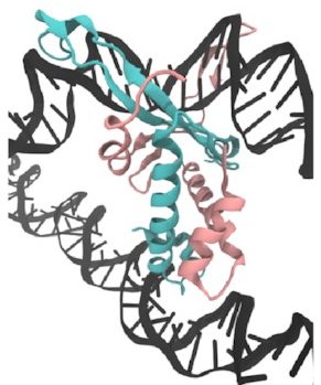
First, we chose a DNA sequence of around 300 base pairs—big enough to see using AFM but just about small enough to simulate in a vaguely acceptable amount of time—containing a binding site for IHF. Then, Sam mixed them together in a test tube or something while I built a sensible initial structure using an experimentally-determined structure of IHF bound to DNA as a starting point. A close-up of that starting structure looks like this:

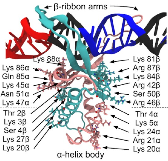
The pink and sort-of-cyan bits are the protein, with a compact body and two arms that give the DNA (the black thing, with some special sequences highlighted in red and blue) a nice hug. The DNA here starts off perfectly straight—it wouldn’t be like that in real life, but it works fine as a starting point for a simulation. The body has lots of positive charges on its sides, which are what all those arrows point to, and the negative charge of DNA means it will naturally be attracted to those positive charges (remember, opposites attract)—that’s how IHF bends DNA so sharply.

And here’s how it looks at the end of a simulation:

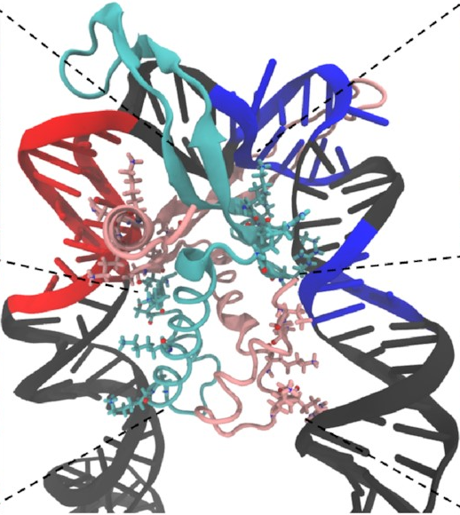
This is exactly what we expected to see—the sharp U-turn I described earlier, with the DNA fully bound to both sides of the protein. This looks a lot like the structures that have already been determined through experimental methods like X-ray crystallography. In fact, we can quantify just how similar they are using something called the root-mean-square deviation (RMSD), effectively the average distance of each atom from where we’d expect it to be. A normal value for a converged simulation might be around 5 Å (the Å symbol represents ångströms—one ångström is about the width of an atom). You’re unlikely to get much less than that purely because atoms are always in motion, jiggling and jostling with thermal energy.

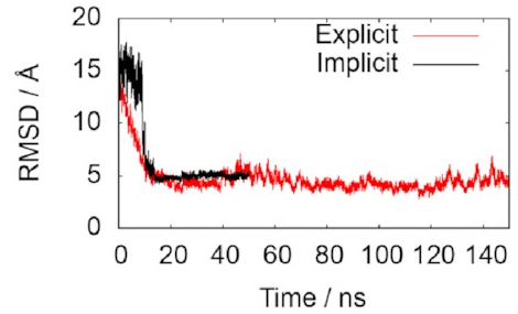
The two lines in this graph represent the two different ways of modelling the water. The important thing is that they both converge on 5 Å, just as we hoped, indicating that the simulations do accurately reproduce the known structure. That means it’s probably safe to keep using them to draw some new conclusions.

Meanwhile, the real pieces of DNA, by now well mixed with IHF, were stuck to a surface and imaged using AFM. Just by looking at the pictures with our eyes, we spotted three different types of structure in both methods:

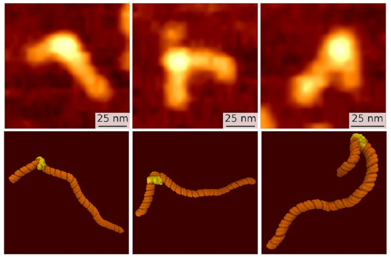
The top row, the slightly fuzzier images, are some of Sam’s AFM images. The bottom row are corresponding frames from my simulations. We both see what looks like the same three states: the fully wrapped one we already knew about (on the right), and two new ones that are a bit less bent. But confirmation bias is a problem: We might just be seeing what we want to see. How can we put a number on it?

Measuring bend angles

The first thing we did was to measure the angle by which the DNA is bent. To do this, we both traced a straight line of about the same length each side of the protein and measured the angle between them. Of course, the AFM image is basically two-dimensional, and the DNA is stuck to a surface, so I projected my simulated structures into a plane—a bit like looking at their shadows—to approximate the same effect.

We measured these angles for every DNA molecule visible in the AFM images and every time step of my simulations (I ran multiple simulations to make sure I sampled as much as possible). The distribution of bend angles in the AFM data looks like this:

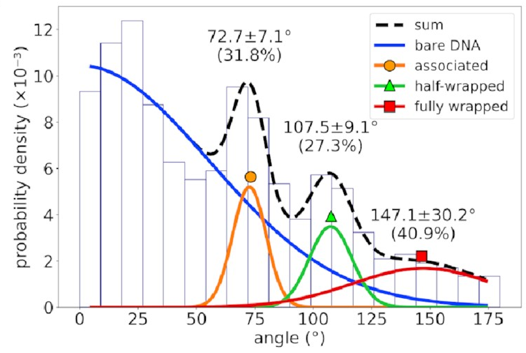
If you’re not familiar with histograms, the horizontal axis represents possible bend angles, and a taller bar means angles in that range are more common. There’s a big mass of barely-bent DNA on the left corresponding to DNA with no IHF bound to it—that’s going to happen in experimental data and can be mostly ignored. To the right of that, however, we see three distinct peaks. That implies we’re seeing something real!

When I do the same analysis on my simulation data, I also get three peaks at very similar bend angles, but there’s a better way to work with atomistic data: hierarchical clustering. Rather than reducing states to a single measurement, like a bend angle, I can directly compare how similar two simulation frames are by measuring the RMSD between them. By doing this for all the frames across all my simulations, and merging the most similar pairs until I was left with a small number of clearly distinct states, I was able to look in detail at the structures of the three different states. These are them:

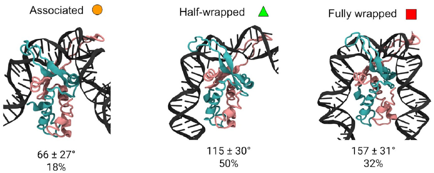
The mean bend angles of these states are pretty close to the values measured from the AFM images! That makes it pretty likely we’re looking at the same thing. These simulations give us the structures of the three states, and tell us exactly how the DNA and protein interact in each one. As well as the original “fully wrapped” state, we have a “half-wrapped” state in which the DNA only binds on one side of the protein—and it’s always the same side (which we’ll call the left)—and another state in which the DNA on each side binds only to the top part of the protein; we called this the “associated” state.

Sequence specificity

There’s something interesting about these binding modes. Well, there are lots of interesting things about them, but there’s one very interesting thing: Why does the left arm sometimes bind without the right arm, but never the other way round?

On the face of it, IHF is a pretty symmetrical protein, but this is decidedly asymmetrical behaviour. Even more interestingly, it has a strong preference for a particular DNA sequence, and that sequence is located on the right arm, which means it doesn’t even interact with the protein in the new states.

For that to make sense, we’d expect to see the associated and half-wrapped states—but not the fully wrapped state—even in pieces of DNA without that sequence. This is where we bring the AFM data back in. For a different DNA sequence without an IHF binding site, the angle distribution looks like this:

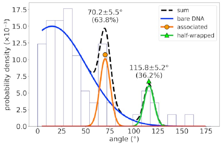
The peaks corresponding to the associated and half-wrapped states are there, clear as day, but the fully wrapped state is missing—just as we expected. This lets us say with a pretty high degree of certainty that these states involve nonspecific binding with no sequence preference. That is, IHF can bind to DNA even if that sequence is missing, but the strong bend for which it is famous is possible only at certain special DNA sites.

Investigating the asymmetry using free-energy calculations

This confirms that our interesting asymmetry is real, but it doesn’t tell us much about it. Just looking at static structures or trajectories doesn’t give us much insight into the binding dynamics. To learn about that, we need to think about free energy.

Free energy is one of the most fundamental concepts in physics and chemistry. The two driving forces of the evolution of physical systems over time are the desire of a system to minimise its internal energy (\(U\)) and maximise its entropy (\(S\)); the balance of these is captured by the (Helmholtz) free energy, \(A\):

\[A = U - T S,\]

where \(T\) is the system’s temperature. A transition between two states can occur spontaneously only if it results in a smaller value of \(A\).

This is very exciting because it tells us which states are stable and which are not. A state with a large free energy compared to those around it won’t occur in nature—and if it does, it won’t last very long. Meanwhile, states with a lower free energy than those around them will probably stay stable for a long time.

What do I mean by a “state”? We can think about all sorts of things that have multiple states: flexible molecules that can take on multiple shapes, maybe, or pairs of molecules that might want to stick together (or might not). In the more human-sized world, a ball placed on the side of a steep hill is in an unstable state, and will quickly roll down to a much more stable position at the bottom of the hill; once it’s there, it’s never going to roll itself back up to the top. A ball perched precisely at the top of the hill might be happy to stay there forever, but just the tiniest nudge will send it tumbling all the way down; a state like this is called “metastable”.

It’s actually very helpful to think in terms of “landscapes” of hills and valleys, where altitude represents free energy. You’ll see some lovely examples of these landscapes shortly.

In principle, I could just run a ridiculously long simulation and keep track of how long the system spends in each state. Since it should spend much more time in states with lower free energy, it’s simple to convert between the two. The problem with that is that the simulation could get stuck in a free-energy valley—it’s very unlikely to climb the sides of the valley in any reasonable amount of time. The probability of the necessary states is just too low. So we’ll sample this one valley really well and never head off to explore the rest of the landscape.

To get around this problem, we can force our simulation to explore the whole landscape by adding an artificial force to literally drag it through all the states. We know how it should behave under the influence of our new force alone; by looking at how the behaviour deviates from this, we can get information about the underlying free-energy landscape. This is called the weighted histogram analysis method, or WHAM.

What we’re interested in is the binding of the DNA to the protein, so it makes sense for our new force to act between a pair of atoms—one towards the bottom of the protein, and one on the DNA. Pulling these closer together forces the DNA and protein to come into contact. Of course, our system has two sides, so we have to do this on both sides. This gives us two dimensions to our free-energy landscape.

Let’s look at the left arm first—that’s the one that binds to the protein in both the fully and half-wrapped states (and partially bound in the associated state too):

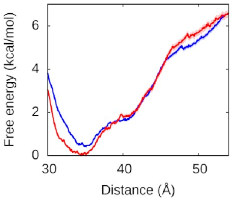
The red line is what happens when we let the right arm bind too; the blue line is what happens when we don’t. As you can see, they’re very similar, which means the left arm’s behaviour doesn’t depend on what the right arm is doing. The other thing you might notice is that this is quite a deep valley—a short distance (that is, a bound state) is very strongly preferred. If the protein and the left DNA arm start about 50 Å apart, they’re going to be strongly attracted to each other and quickly roll into the bound state at the bottom of the valley.

What about the right arm? That looks more like this:

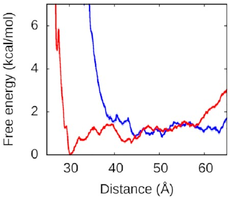
Now, this is interesting. The right arm doesn’t have the same kind of deep free-energy valley as the left one. The right half of that graph is mostly flat, with the only lumps and bumps being seemingly random fluctuations on the order of thermal noise. To the left of the graph, we see the expected sharp rise as the protein and DNA get pushed too close together—two objects can’t occupy the same space and will resist very strongly any attempts to make them. But we see that we reach this point much sooner along the blue line, when the left arm is held away from the protein, than along the red line, when the left arm is free to bind.

Astute readers might have figured out what’s going on here. We’ve explained why we never see the right arm binding without the left. Until the left arm binds, there’s a physical obstacle in the way. If we overlay the structures of the fully wrapped and associated states, we can see what’s going on here:

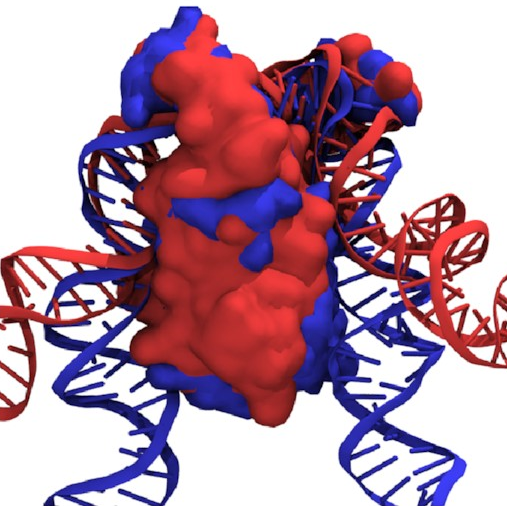
Here, the fully wrapped state is in blue and the associated state in red. In the associated state, the protein body is noticeably tilted; the right arm would have to bend significantly to bind any farther down the protein. In the fully wrapped state, things have straightened up and both arms can bind without bending. DNA is quite a rigid polymer, so this amounts to a rule preventing the right arm from binding first.

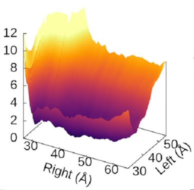
The scale of the asymmetry might be easier to grasp if we view the landscape in 3D, which really emphasises how steep the potential for the left arm is compared to the flat right arm:

We could also look at where our three states sit on this landscape. It turns out—as we’d hope—that they’re associated with valleys and flat regions:

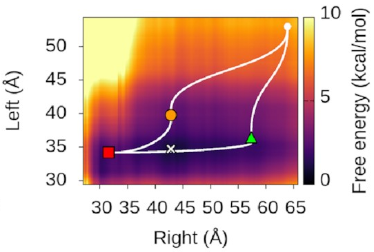
They’re also really nice to look at!

DNA bridging by IHF

While we were doing all this, something else interesting turned up in the AFM images. You may recall that IHF stabilises biofilms by holding pieces of DNA together. Well, we started getting pictures like these:

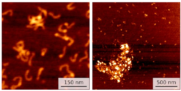
On the left, you can see a few small clusters of DNA with bright spots showing IHF holding them together. On the right is data for a different sequence with not one but three IHF binding sites: a huge blob of DNA and IHF!

This seems to line up with what happens in biofilms. IHF is clearly holding multiple pieces of DNA together. So I ran some simulations to investigate.

First, I set up this initial bridged structure by sort of encouraging another piece of DNA to get close to the protein:

Then, I used WHAM again to pull the second piece of DNA away. The resulting free-energy landscape looks like this:

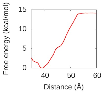
That’s a nice deep well again: IHF loves to form bridges! about 50 Å is going to be attracted and eventually bind to the bottom of the protein in a structure a lot like the one above. Understanding this could help us to understand how to disrupt IHF’s role in biofilms and treat bacterial infections better.

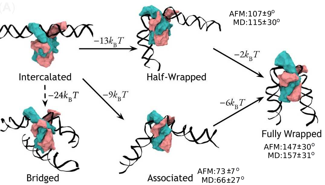
A complete model of IHF binding, bending, & bridging

We now have enough information to produce a complete model of IHF’s interactions with DNA. Here it is:

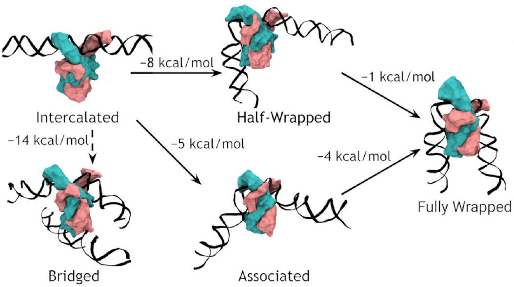
So, IHF first binds to straight DNA, which we’ve labelled the “intercalated” state in the diagram, because part of the protein is intercalated (inserted between DNA base pairs); this isn’t really a real state, because our energy landscapes predict that it shouldn’t last very long. If there’s some other DNA nearby, it will really want to form a bridge. Otherwise, it will progress to either the associated or the half wrapped state; it’s not entirely clear how it picks, and there’s almost certainly a random element, but the half-wrapped state seems to be preferred. It doesn’t look like it should be possible to move between these two states, but they can both eventually progress further into the fully wrapped state.

If you’ve made it this far, hopefully you agree it’s really cool that we can figure all of this out, especially by combining simulations and experiments in this manner. I think this is a really promising approach that could be super valuable for other studies in the future, and I’d encourage you to try and break down any disciplinary barriers you can because that’s where all the most interesting stuff is hidden.

I’m always happy to talk more about science, so do get in touch if you’re interested. I’ll be Tweeting about this so you’re welcome to reply there, and there’s a comment section below.

Thank you for your time.

1. Mad, innit? ↩

2. That’s not quite true—some of your cells, such as red blood cells, don’t contain any DNA, but that doesn’t really fix anything. ↩

3. and lots and lots… ↩

4. Unfortunately, these are nowhere near as exciting and useful as the ones that block phaser fire, and look more like this. ↩

5. Thales here makes his second appearance in as many posts, purely coïncidentally. ↩

6. Actually, we don’t usually use cubes, and a whole section of my thesis is devoted to the interesting properties of the truncated octahedron, but that’s not really important. ↩

7. Sometimes it’s okay to set a cutoff distance beyond which the interactions are basically zero so there’s no need to calculate them, but often not, and we still need to consider a lot of atoms either way. ↩

---

Citation & images: Yoshua S B, Watson G D et al. 2021 Nucleic Acids Res. gkab641 doi:10.1093/nar/gkab641 (CC-BY)